Advanced Lane Finding Project
Overview
The goals / steps of this project are the following:
- Compute the camera calibration matrix and distortion coefficients given a set of chessboard images.
- Apply a distortion correction to raw images.
- Use color transforms, gradients, etc., to create a thresholded binary image.
- Apply a perspective transform to rectify binary image (“birds-eye view”).
- Detect lane pixels and fit to find the lane boundary.
- Determine the curvature of the lane and vehicle position with respect to center.
- Warp the detected lane boundaries back onto the original image.
- Output visual display of the lane boundaries and numerical estimation of lane curvature and vehicle position.
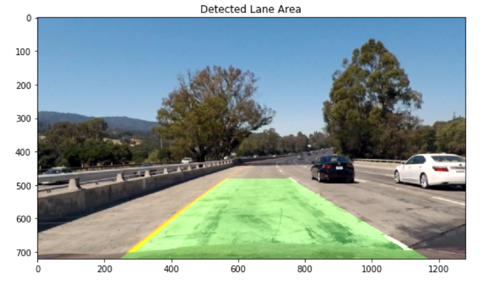
Rubric Points
The code for this project is contained in the IPython notebook: “Advanced_Lane_Finding.ipynb”
Writeup / README
Camera Calibration
Images taken through camera lenses tend to introduce image distortion, which occurs when a camera looks at 3D objects in the real world and transforms them into a 2D image that isn’t exact. There are many different types of image distortion, but radial distortion is the most common.
With this in mind the camera must be calibrated to account for possible distortion in an image. To calibrate a camera for distortion pictures of known shapes must be used and it is recommended to use at least 20 images taken at different angles and distances to obtain a more accurate calibration.
Images of a chessboard was used because of it’s regular high contrast pattern which makes it easy to detect automatically and it is easy to identify what a distorted chessboard looks like. Using these calibration images we can create object and image points. Image points are the coordinates of the corners in a 2D image which are mapped to the known 3D coordinates of the real undistorted image corners (x, y, z), object points, where z is zero for every point because the board is on a flat image plane. These object points will be the same for each calibration image because they are just the known coordinates of the object corners for a 9x6 chessboard.
The OpenCV function findChessboardCorners() allows for automatic detection of corners. Each time a corner is successfully detected the points are appended to an objpoint array and the (x,y) position of the corner is appended to an imgpoint array. The detected corners are then automatically drawn on the chessboard image using the function drawChessboardCorners() resulting in the image below:
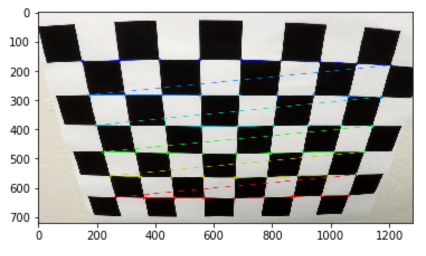
These detected image and object points are then used in the function calibrateCamera() in order to obtain a calibration matrix and the distortion coefficients.
Pipeline (single images)
1. Distortion correction
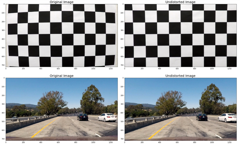
Distortion can change the apparent size and shape of an object in an image, cause an objects appearance to change depending on where it is in the FOV and make objects appear closer or farther away than they actually are. To avoid these things, the distortion coefficients and calibration matrix from above is used to apply a distortion correction using the function undistort() which maps the distorted points on an image to undistorted points.

2. Gradients and Color transforms
Now that the camera is calibrated for distortion and the raw images have been undistorted, color transforms and gradients can be used to create a threshold binary image.
First, I compute the gradient by essentially taking the derivative of the undistorted image in the x and y direction respectively using the OpenCV function Sobel() . Taking the gradient in the x direction emphasizes edges closer to vertical. Alternatively, taking the gradient in the y direction emphasizes edges closer to horizontal.
These gradients are than set between binary thresholds to select pixels based on the strength of the gradient.
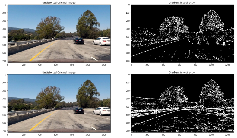
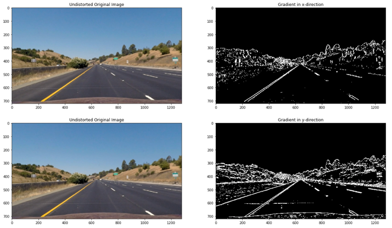
Although both gradients pick up the lane lines well, taking the gradient in the x direction does a better job. In order to see the maximum rate of change at each point, the magnitude of the gradient was computed as seen below:
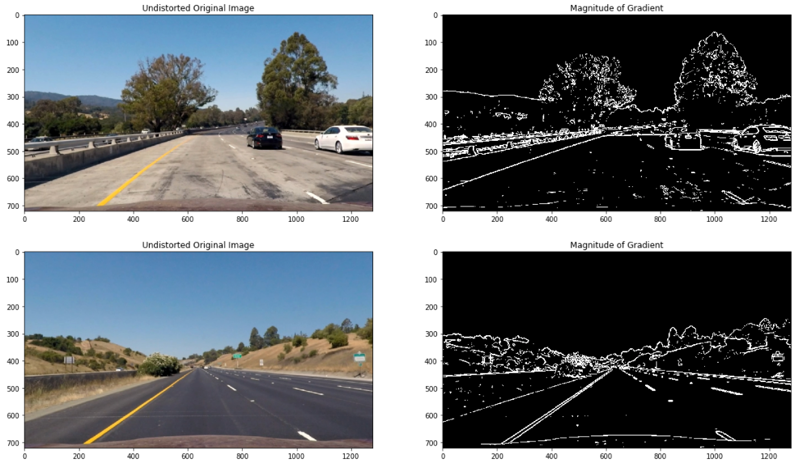
Gradient magnitude is basis for the Canny edge detection, and is why Canny works well for picking up all edges, but since I am detecting lane lines I am only interested in edges of a particular orientation. Now I must explore the direction, or orientation, of the gradient so I computed the direction of the gradient as seen below. Each pixel of the resulting image contains a value for the angle of the gradient away from horizontal in units of radians, covering a range of −π/2 to π/2. An orientation of 0 implies a vertical line and orientations of +/−π/2 to +/−π/2 imply horizontal lines.
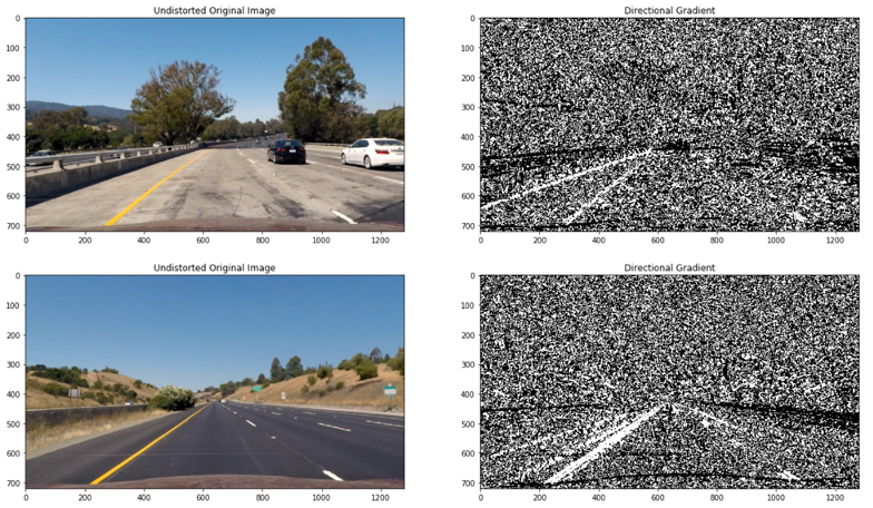
The gradient computations above require the undistorted image to be converted from RGB/BGR to GRAYSCALE and in doing this conversion, valuable color information is lost. To obtain more information about the image, a more robust color space is used, HLS.
In this color space the S refers to saturation, the measurement of colorfulness. As colors get lighter and closer to white, they have a lower saturation value, whereas colors that are the most intense, like a bright primary color, have a high saturation value. The S channel picks up the lines well as seen below
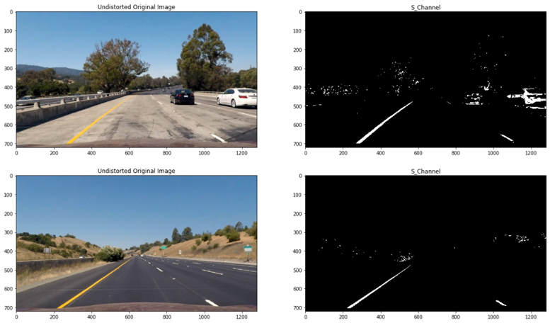
To get a more robust binary image where the lane lines are clearly visible, color and gradient thresholds are combined. This will also help with detecting the lane lines under varying degrees of daylight and shadow.
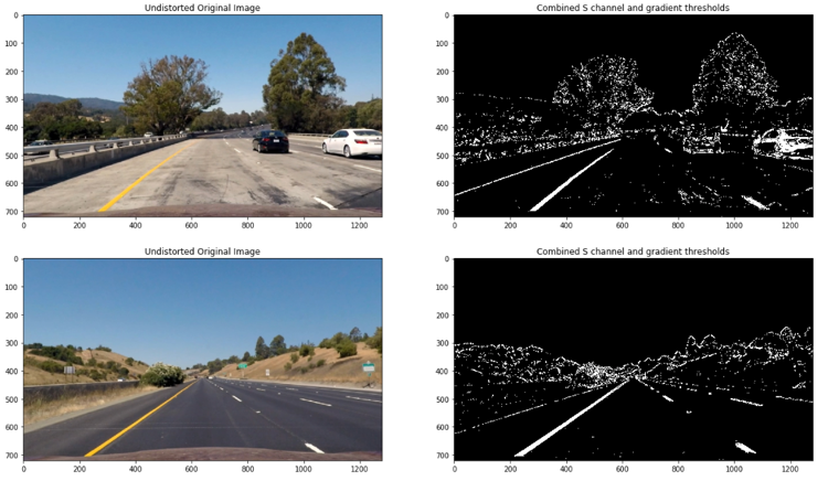
3. Perspective transform
A perspective transform maps the points in a given image to different, desired, image points with a new perspective. In our case the new perspective is a top-down view, or “birds-eye” view that lets us view a lane from above. This transform is particularly important when measuring the curvature of the lines.
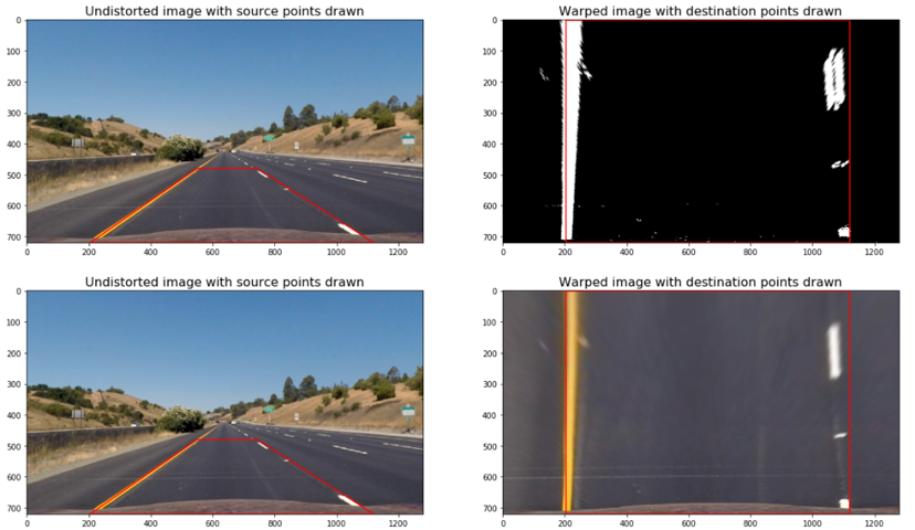
In order to perform the transform I defined four source points that form the trapezoid in the right side image below and four destination points of where I want the source points to appear after the transformation, or warp.
| Source | Destination | |
|---|---|---|
| Bottom Left | 205, 720 | 205, 720 |
| Bottom Right | 1120, 720 | 1120, 720 |
| Top Right | 745, 480 | 1120, 0 |
| Top Left | 550, 480 | 205, 0 |
These source and destination points are used in the function
getPerspectiveTransform()to obtain the transformation matrix, M. M is then applied to the function warpPerspective() to warp the image to a top-down view and the destination points are then drawn on to the image.
The points selected above are tested on a straight line image first as seen below
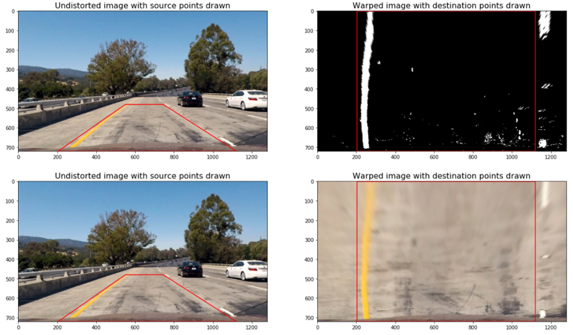
And then applied to an image with curves as seen below
4. Lane Detection
After applying calibration, thresholding, and a perspective transform to the image, I have a binary image where the lane lines stand out clearly, but I still need to decide explicitly which pixels are part of the lines and which belong to the left line and which belong to the right line.
Two different methods were used to detect the lane lines: sliding window search and search from prior.
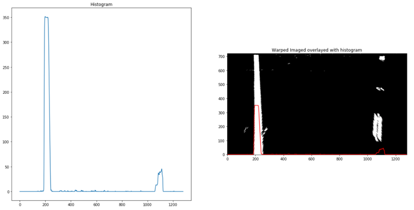
First, a histogram of where the binary activations occur across the image is computed and split into two sides, one for each line. The two highest peaks from the histogram provides a starting point for determining where the lane lines are.
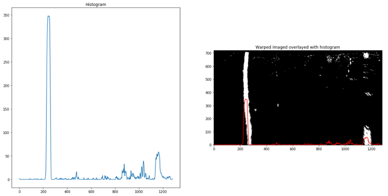
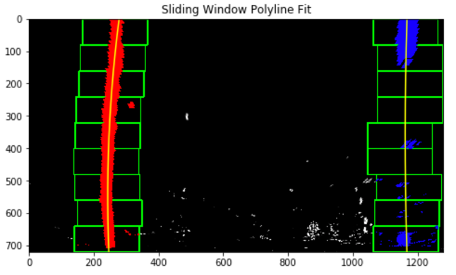
A sliding window is then used to move upward in the image (further along the road) to determine where the lane lines go. A second-order polynomial is also fitted to the lanes detected from the histogram as seen below. The number of sliding windows are represented by the green rectangles and the size of each window is defined by the parameter “margin”.
The second method used was a “search from prior”. Instead of starting fresh on every frame and doing a blind search again this method will search a margin around the previous lane line position. Once the lane lines are identified in the first frame, a highly targeted search is then performed for the next frame.
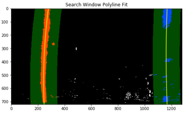
Sanity checks are performed to ensure that the lines are the correct distance, at least between 3.3m and 3.7 m, and that they are roughly parallel between the width of the line.
If any of my sanity checks reveal that the lane lines detected are problematic I simply retain the previous positions from the frame prior and step to the next frame to search again. If lines are lost for several frames in a row, the search is started from scratch using a sliding window.
5. Radius of Curvature
Since a perspective transform has been performed above, computing the radius of curvature for each lane line by using the second order polynomial that were fitted above is made easy.
By M. Bourne We can draw a circle that closely fits nearby points on a local section of a curve, as shown below:
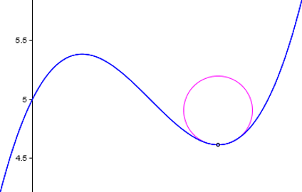
The radius of curvature of the curve at a particular point is defined as the radius of the approximating circle that could be tangent to the lane lines. This radius changes as we move along the curve.
The radius of curvature at any point x of the function x=f(y) is given as follows:
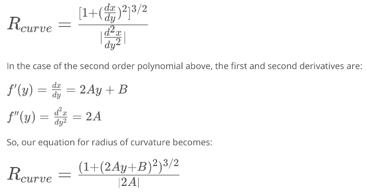
We assume the camera is mounted at the center of the car, such that the lane is the midpoint at the bottom of the image between two lines so we must account for the vehicles distance from the center of the lane, the offset.
6. Result
Finally, we warp the detected lane boundaries back onto the original image to get the result below.

Numerical estimation of lane curvature and vehicle position are then added to the output to create the final image below.

Pipeline (video)
Here’s a link to my final video video
Discussion
Potential shortcomings
- Unexpected inputs (previous lane line markings, shadows, and varying pavement colors) that cause the pipeline to make a few mistakes.
- The pipeline may also not do well if objects cover the lane line.
- Sanity checks don’t provide enough verification of the lane which causes the detection region to sometimes fall short of the lane distance on curves.
Possible Improvements
There is much room for improvements to this project:
- Use of heat maps and other color spaces to retain more information about an image.
- Implementing more sanity checks to ensure detected lanes are valid. e.g. coefficient check for change in fits, if change is too sharp then the lane detection may have been off.
- Use detected corners from the camera calibration to find the source and destination points for the perspective transform.
- Add yellow and white color mask to better detect the lanes